Chapter 10 Estimating With Confidence Reading Guide Answers

Conviction Intervals
In Chapter 9, we developed a theory of repeated samples. Simply what does this mean for your data assay? If you only take one sample in front of you, how are you supposed to empathize properties of the sampling distribution and your estimators? In this chapter we use the mathematical theory nosotros introduced in Sections 9.iv.ane - 9.7 to tackle this question.
Needed Packages
Let's load all the packages needed for this affiliate (this assumes y'all've already installed them). If needed, read Department 1.3 for information on how to install and load R packages.
Combining an estimate with its precision
A conviction interval gives a range of plausible values for a parameter. Information technology allows united states of america to combine an guess (east.g. \(\bar{10}\)) with a measure of its precision (i.e. its standard error). Conviction intervals depend on a specified confidence level (e.g. 90%, 95%, 99%), with higher confidence levels corresponding to wider conviction intervals and lower confidence levels corresponding to narrower confidence intervals.
Usually nosotros don't merely brainstorm sections with a definition, merely conviction intervals are simple to ascertain and play an important role in the sciences and whatever field that uses data.
You can think of a confidence interval every bit playing the role of a internet when fishing. Using a single point-estimate to estimate an unknown parameter is like trying to take hold of a fish in a murky lake with a single spear, and using a confidence interval is like fishing with a net. We can throw a spear where we saw a fish, but we volition probably miss. If we toss a net in that area, we have a good run a risk of catching the fish. Analogously, if we report a point judge, we probably won't hitting the verbal population parameter, but if we written report a range of plausible values based effectually our statistic, we have a good shot at catching the parameter.
Sampling distributions of standardized statistics
In order to construct a confidence interval, nosotros need to know the sampling distribution of a standardized statistic. We can standardize an guess by subtracting its hateful and dividing by its standard error:
\[STAT = \frac{Approximate - Mean(Gauge)}{SE(Judge)}\] While we have seen that the sampling distribution of many common estimators are normally distributed (meet Table 9.6), this is non always the case for the standardized estimate computed past \(STAT\). This is because the standard errors of many estimators, which appear on the denominator of \(STAT\), are a function of an additional estimated quantity – the sample variance \(southward^ii\). When this is the case, the sampling distribution for STAT is a t-distribution with a specified degrees of freedom (df). Table 10.1 shows the distribution of the standardized statistics for many of the common statistics we have seen previously.
| Statistic | Population parameter | Estimator | Standardized statistic | Sampling distribution of standardized statistic |
|---|---|---|---|---|
| Proportion | \(\pi\) | \(\widehat{\pi}\) | \(\frac{\lid{\pi} - \pi}{\sqrt{\frac{\hat{\pi}(1-\hat{\pi})}{n}}}\) | \(N(0,1)\) |
| Mean | \(\mu\) | \(\overline{x}\) or \(\widehat{\mu}\) | \(\frac{\bar{x} - \mu}{\frac{s}{\sqrt{n}}}\) | \(t(df = northward-i)\) |
| Difference in proportions | \(\pi_1 -\pi_2\) | \(\widehat{\pi}_1 - \widehat{\pi}_2\) | \(\frac{(\hat{\pi}_1 - \lid{\pi}_2) - {(\pi_1 - \pi_2)}}{\sqrt{\frac{\chapeau{\pi}_1(1-\hat{\pi}_1)}{n_1} + \frac{\chapeau{\pi}_2(i - \hat{\pi}_2)}{n_2}}}\) | \(N(0,1)\) |
| Deviation in ways | \(\mu_1 - \mu_2\) | \(\overline{x}_1 - \overline{x}_2\) | \(\frac{(\bar{x}_1 - \bar{x}_2) - (\mu_1 - \mu_2)}{\sqrt{\frac{s_1^2}{n_1} + \frac{s_2^2}{n_2}}}\) | \(t(df = min(n_1 - 1, n_2 - 1))\) |
| Regression intercept | \(\beta_0\) | \(b_0\) or \(\widehat{\beta}_0\) | \(\frac{b_0 - \hat{\beta}_0}{\sqrt{s_y^2[\frac{i}{n} + \frac{\bar{x}^ii}{(n-i)s_x^ii}]}}\) | \(t(df = due north-2)\) |
| Regression slope | \(\beta_1\) | \(b_1\) or \(\widehat{\beta}_1\) | \(\frac{b_1 - \beta_1}{\sqrt{\frac{s_y^2}{(northward-one)s_x^two}}}\) | \(t(df = n-2)\) |
If in fact the population standard variance was known and didn't have to be estimated, we could supersede the \(s^2\)'south in these formulas with \(\sigma^ii\)'s, and the sampling distribution of \(STAT\) would follow a \(Due north(0,1)\) distribution.
Confidence Interval with the Normal distribution
If the sampling distribution of a standardized statistic is normally distributed, and so we can use properties of the standard normal distribution to create a confidence interval. Recall that in the standard normal distribution:
- 90% of values are between -1.645 and +ane.645.
- 95% of the values are between -i.96 and +1.96.
- 99% of values are between -2.575 and +2.575
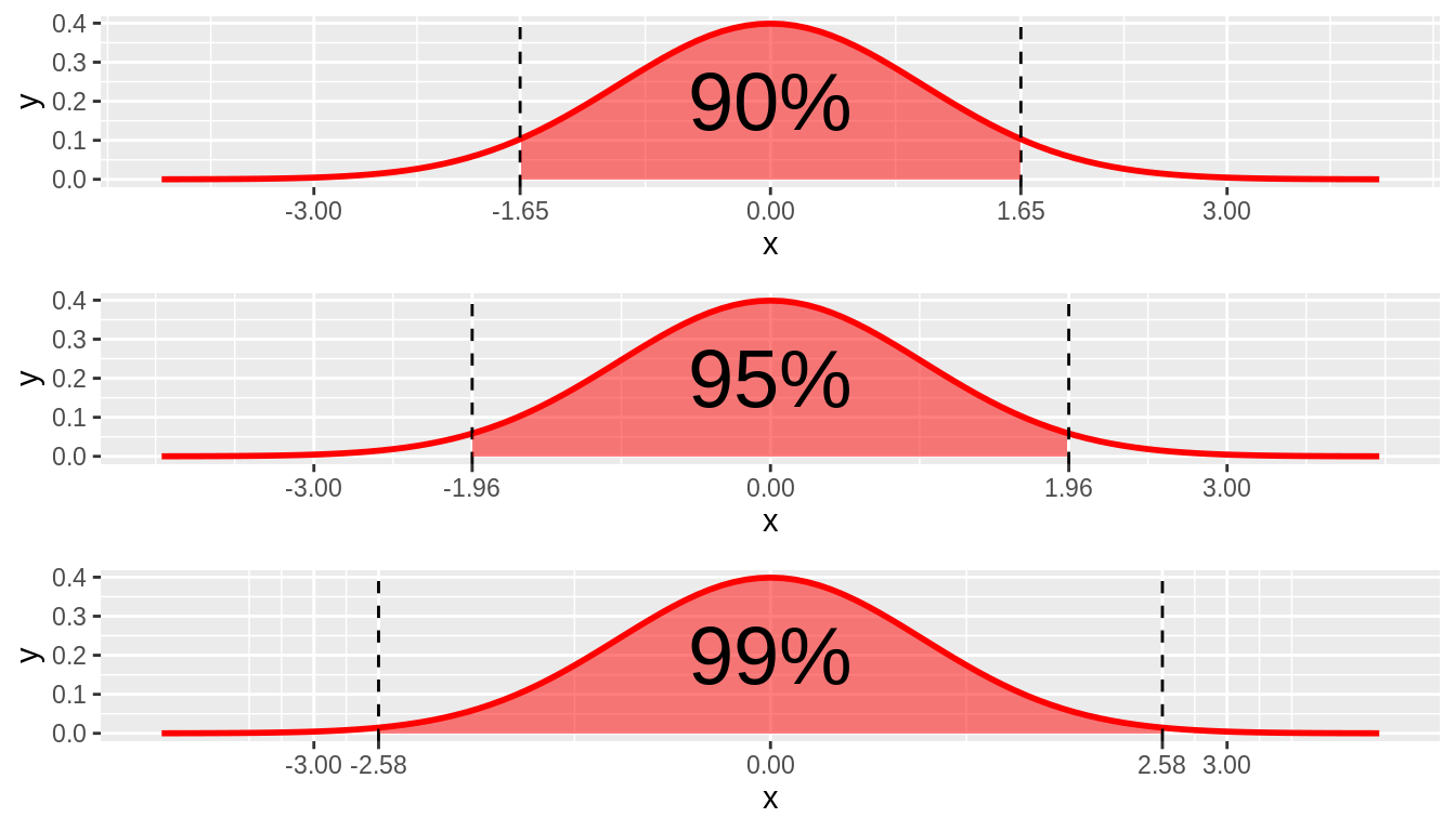
FIGURE 10.1: N(0,i) 95% cutoff values
Using this, we tin define a 95% confidence interval for a population parameter as, \[Estimate \ \pm 1.96*SE(Guess),\] or written in interval notation as \[[Estimate \ \ – \ 1.96*SE(Estimate),\ \ \ Guess + one.96*SE(Estimate)]\]
For case, a 95% conviction interval for the population mean \(\mu\) can be constructed based upon the sample hateful as, \[[\bar{x} - 1.96\frac{\sigma}{\sqrt{n}}, \ \bar{ten} + i.96\frac{\sigma}{\sqrt{northward}}],\] when the population standard deviation is known. Nosotros will show later on in this section how to construct a conviction interval for the mean using a t-distribution when the population standard deviation is unknown.
Let's return to our football fan instance. Imagine that we have data on the population of 40,000 fans, their ages and whether or not they are cheering for the home team. This faux information exists in the data frame football_fans.
We come across that the average age in this population is \(\mu =\) 30.064 and the standard deviation is \(\sigma =\) viii.017.
mu sigma 1 thirty.ane 8.02 Let'due south take a sample of 100 fans from this population and compute the average age, \(\bar{10}\) and its standard error \(SE(\bar{x})\).
n xbar sigma SE_xbar 1 100 29.7 8.02 0.802 Because the population standard deviation is known and therefore the standarized mean follows a \(N(0,1)\) distribution, we tin can construct a 95% confidence interval for \(\bar{10}\) by
\[29.7 \pm 1.96*\frac{8.02}{\sqrt{100}},\] which results in the interval \([28.1, 31.iii]\).
lower upper 1 28.ane 31.three A few properties are worth keeping in heed:
- This interval is symmetric. This symmetry follows from the fact that the normal distribution is a symmetric distribution. If the sampling distribution does not follow the normal or t-distributions, the confidence interval may non exist symmetric.
- The multiplier ane.96 used in this interval corresponding to 95% comes direct from backdrop of the normal distribution. If the sampling distribution is non normal, this multiplier might be different. For case, this multiplier is larger when the distribution has heavy tails, as with the t-distribution. The multiplier volition also be different if you desire to use a level of confidence other than 95%. We will discuss this further in the adjacent section.
- Rather than simply reporting our sample mean \(\bar{x} = 29.7\) as a unmarried value, reporting a range of values via a conviction interval takes into business relationship the uncertainty associated with the fact that we are observing a random sample and not the whole population. We saw in Chapter ix that there is sampling variation inherent in taking random samples, and that (fifty-fifty unbiased) estimates volition non exist exactly equal to the population parameter in every sample. Nosotros know how much dubiety/sampling variation to account for in our confidence intervals because we have known formulas for the sampling distributions of our estimators that tell us how much we expect these estimates to vary across repeated samples.
General Form for Constructing a Conviction Interval
In general, we construct a conviction interval using what we know about an estimator's standardized sampling distribution. Above, we used the multiplier 1.96 because we know that \(\frac{\bar{x} - \mu}{\frac{\sigma}{\sqrt{n}}}\) follows a standard Normal distribution, and nosotros wanted our "level of confidence" to be 95%. Note that the multiplier in a confidence interval, often called a critical value, is just a cutoff value from either the \(t\) or standard normal distribution that corresponds to the desired level of confidence for the interval (e.g. ninety%, 95%, 99%).
In general, a confidence interval is of the course:
\[\text{Estimate} \pm \text{Critical Value} * SE(\text{Gauge})\]
In order to construct a conviction interval you need to:
- Summate the estimate from your sample
- Calculate the standard error of your judge (using formulas plant in Table 9.half dozen)
- Determine the advisable sampling distribution for your standardized estimate (usually \(t(df)\) or \(N(0,1)\). Refer to Table 10.1)
- Make up one's mind your desired level of confidence (e.m. 90%, 95%, 99%)
- Use 3 and 4 to determine the correct critical value
Finding critical values
Suppose nosotros have a sample of \(n = 20\) and are using a t-distribution to construct a 95% confidence interval for the hateful. Remember that the t-distribution is characterized by its degrees of freedom; here the appropriate degrees of liberty are \(df = due north - 1 = nineteen\). We can find the appropriate disquisitional value using the qt() role in R. Remember that in guild for 95% of the data to autumn in the middle, this ways that two.v% of the data must fall in each tail, respectively. We therefore desire to notice the critical value that has a probability of 0.025 to the left (i.e. in the lower tail).
[i] -2.09 Note that because the t-distribution is symmetric, we know that the upper cutoff value volition be +2.09 and therefore information technology's not necessary to calculate information technology separately. For demonstration purposes, however, we'll prove how to calculate it in two ways in R: by specifying that we want the value that gives two.5% in the upper tail (i.e. lower.tail = FALSE) or by specifying that we want the value that gives 97.5% in the lower tail. Note these ii are logically equivalent.
[1] 2.09 [one] 2.09 Importantly, changing the degrees of freedom (by having a different sample size) volition change the critical value for the t-distribution. For case, if instead we have \(due north = 50\), the correct disquisitional value would exist \(\pm 2.01\). The larger the sample size for the t-distribution, the closer the critical value gets to the corresponding critical value in the North(0,1) distribution (in the 95% case, 1.96).
[1] -ii.01 Recall that the critical values for 99%, 95%, and 90% conviction intervals for the \(N(0,1)\) are given by \(\pm 2.575, \pm ane.96,\)and \(\pm 1.645\) respectively. These are likely numbers you will memorize from using often, but they can besides be calculated using the rnorm() role in R.
[ane] -2.58 [1] -1.96 [1] -ane.64 Case
Returning to our football fans example, let'southward assume we don't know the truthful population standard divergence \(\sigma\), but instead we have to estimate information technology by \(south\), the standard divergence calculated in our sample. This means we need to calculate \(SE(\bar{x})\) using \(\frac{s}{\sqrt{n}}\) instead of \(\frac{\sigma}{\sqrt{north}}\).
n xbar s SE_xbar 1 100 29.7 7.78 0.778 In this instance, we should use the t-distribution to construct our confidence interval considering - refering back to Table 10.ane - we know \(\frac{\bar{ten} - \mu}{\frac{s}{\sqrt{n}}} \sim t(df = northward-1)\). Think that nosotros took a sample of size \(n = 100\), so our degrees of freedom here are \(df = 99\), and the appropriate critical value for a 95% confidence interval is -1.984.
[ane] -1.98 Therefore, our conviction interval is given by
\[29.7 \pm 1.98*\frac{7.78}{\sqrt{100}},\] which results in the interval \([28.i, 31.ii]\).
lower upper 1 28.1 31.2 Interpreting a Confidence Interval
Like many statistics, while a confidence interval is fairly straightforward to construct, it is very like shooting fish in a barrel to translate incorrectly. In fact, many researchers – statisticians included – get the interpretation of confidence intervals wrong. This goes back to the idea of counterfactual thinking that nosotros introduced previously: a conviction interval is a property of a population and estimator, non a particular sample. It asks: if I constructed this interval in every possible sample, in what percentage of samples would I correctly include the true population parameter? For a 99% confidence interval, this answer is 99% of samples; for a 95% confidence interval, the reply is 95% of samples, etc.
To see this, let's render to the football fans example and consider the sampling distribution of the sample hateful historic period. Call up that nosotros have population data for all 40,000 fans. Below we take ten,000 repeated samples of size 100 and display the sampling distribution of the sample mean in Figure ten.2. Recall that the true population mean is thirty.064
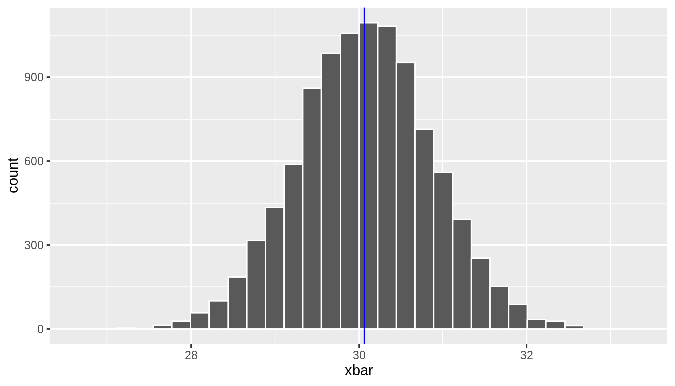
FIGURE 10.ii: Sampling Distribution of Boilerplate Historic period of Fans at a Football
Assume that the sample we really observed was replicate = 77, which had \(\bar{x} =\) 29.7. If we used this sample mean to construct a 95% conviction interval, the population mean would be in this interval, right? Figure ten.iii shows a confidence interval shaded effectually \(\bar{ten} =\) 29.7, which is indicated by the red line. This confidence interval successfully includes the truthful population mean.
# A tibble: 1 ten 2 lower upper <dbl> <dbl> 1 28.1 31.two 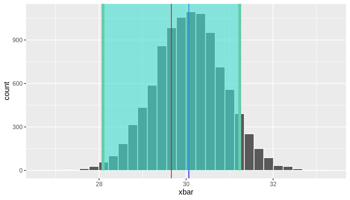
FIGURE 10.three: Confidence Interval shaded for an observed sample hateful of 29.viii
Assume at present that we were unlucky and drew a sample with a mean far from the population hateful. One such example is replicate = 545, which had \(\bar{x} =\) 32.3. In this case, is the population hateful in this interval? Figure 10.4 displays this scenario.
# A tibble: i x 2 lower upper <dbl> <dbl> ane 30.7 33.eight 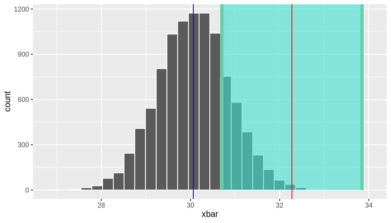
FIGURE 10.four: Confidence Interval shaded for an observed sample mean of 32.iii
In this case, the confidence interval does not include the true population mean. Chiefly, remember that in real life we simply have the data in front of united states from ane sample. We don't know what the population mean is, and we don't know if our estimate is the value virtually to the mean (Figure ten.3 ) or far from the mean (Figure x.4 ). Also recall replicate = 545 was a legitimate random sample fatigued from the population of xl,000 football fans. Just by chance, it is possible to discover a sample mean that is far from the true population mean.
We could compute 95% confidence intervals for all 10,000 of our repeated samples, and we would expect approximately 95% of them to contain the true hateful; this is the definition of what it ways to exist "95% confident" in statistics. Another manner to think about it, when constructing 95% conviction intervals, we await that we'll just cease upwards with an "unlucky" sample- that is, a sample whose mean is far enough from the population mean such that the confidence interval doesn't capture it - just v% of the time.
For each of our 10,000 samples, let's create a new variable captured_95 to indicate whether the true population mean \(\mu\) is captured between the lower and upper values of the confidence interval for the given sample. Let's wait at the results for the showtime 5 samples.
# A tibble: 5 x 8 replicate xbar sigma north SE_xbar lower upper captured_95 <int> <dbl> <dbl> <int> <dbl> <dbl> <dbl> <lgl> 1 1 30.vii 8.02 100 0.802 29.2 32.three TRUE 2 two 29.7 eight.02 100 0.802 28.two 31.3 Truthful 3 3 29.v 8.02 100 0.802 28.0 31.i TRUE 4 four 30.vii 8.02 100 0.802 29.1 32.ii TRUE 5 v thirty.two 8.02 100 0.802 28.half-dozen 31.7 Truthful We come across that each of the first 5 confidence intervals do comprise \(\mu\). Permit'southward look beyond all 10,000 confidence intervals (from our 10,000 repeated samples), and come across what proportion contain \(\mu\).
# A tibble: 1 x 1 `sum(captured_95)/n()` <dbl> i 0.951 In fact, 95.06% of the 10,000 do capture the true mean. If we were to have an infinite number of repeated samples, we would see this number approach exactly 95%.
For visualization purposes, we'll take a smaller subset of 100 of these confidence intervals and display the results in Figure 10.5. In this smaller subset, 96 of the 100 95% confidence intervals incorporate the true population hateful.
CI_subset <- sample_n(CIs_football_fans, 100) %>% mutate(replicate_id = seq(1 : 100)) ggplot(CI_subset) + geom_point(aes(x = xbar, y = replicate_id, color = captured_95)) + geom_segment(aes(y = replicate_id, yend = replicate_id, x = lower, xend = upper, color = captured_95)) + labs(x = expression("Historic period"), y = "Replicate ID", title = expression(paste("95% percentile-based confidence intervals for ", mu, sep = ""))) + scale_color_manual(values = c("blue", "orange")) + geom_vline(xintercept = mu, color = "reddish") 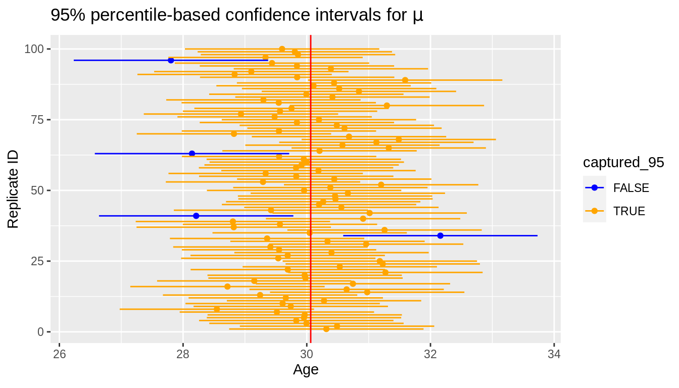
FIGURE 10.5: Confidence Interval for Boilerplate Historic period from 100 repeated samples of size 100
What if nosotros instead constructed 90% conviction intervals? That is, we instead used 1.645 as our critical value instead of 1.96.
# A tibble: one x i `sum(captured_90)/n()` <dbl> 1 0.901 Equally expected, when we use the 90% disquisitional value, approximately 90% of the confidence intervals comprise the true mean. Annotation that considering we are using a smaller multiplier (1.645 vs. 1.96), our intervals are narrower, which makes it more likely that some of our intervals will not capture the true mean. Recollect back to the fishing analogy: you will probably capture the fish fewer times when using a small internet versus a large internet.
Margin of Fault and Width of an Interval
Call up that nosotros said in general, a confidence interal is of the form:
\[\text{Estimate} \pm \text{Critical Value} * SE(\text{Judge})\]
The second element of the confidence interval (\(\text{Disquisitional Value} * SE(\text{Estimate}\)) is frequently called the margin of error. Therefore, another general way of writing the conviction interval is \[\text{Gauge} \pm \text{Margin of Error}\]
Note that as the margin of mistake decreases, the width of the interval also decreases. But what makes the margin of fault decrease? We've already discussed one fashion: by decreasing the level of confidence. That is, using a lower conviction level (eastward.m. 90% instead of 95%) volition decrease the disquisitional value (e.g. 1.645 instead of 1.96) and thus effect in a smaller margin of mistake and narrower confidence interval.
In that location is a trade-off hither between the width of an interval and the level of confidence. In full general we might recollect narrower intervals are preferrable to wider ones, merely by narrowing your interval, you are increasing the chance that your interval volition not capture the true mean. That is, a 90% confidence interval is narrower than a 95% confidence interval, simply it has a ten% hazard of missing the hateful as opposed to just a 5% gamble of missing information technology. The trade-off in the other direction is this: a 99% confidence level has a higher chance of capturing the truthful mean, just it might be too broad of an interval to be practically useful. This Garfield comic demonstrates how at that place are drawbacks to using a college-confidence (and therefore wider) interval.

A second style y'all tin decrease the margin of error is by increasing sample size. Recall that all of our formulas for standard errors involve \(n\) on the denominator (run across Table 9.vi ), so by increasing sample size on the denominator, nosotros decrease our standard error. We also saw this demonstrated via simulations in Section 9.6. Because our margin of error formula involves standard error, increasing the sample size decreases the standard mistake and thus decreases the margin of error. This fits with our intuition that having more infomation (i.eastward. a larger sample size) volition give us a more precise estimate (i.e. a narrower confidence interval) of the parameter nosotros're interested in.
Instance: Ane proportion
Let's revisit our exercise of trying to judge the proportion of red assurance in the bowl from Chapter 9. Nosotros are at present interested in determining a confidence interval for population parameter \(\pi\), the proportion of balls that are red out of the total \(Northward = 2400\) cerise and white assurance.
We will use the showtime sample reported from Ilyas and Yohan in Subsection 9.2.3 for our point guess. They observed 21 red balls out of the fifty in their shovel. This information is stored in the tactile_shovel1 data frame in the moderndive packet.
# A tibble: l x 1 colour <chr> one white 2 red 3 red 4 ruddy 5 ruby-red vi red seven carmine 8 white 9 red 10 white # … with 40 more rows Observed Statistic
We can use our data wrangling tools to compute the proportion that are red in this information.
# A tibble: ane 10 three n pi_hat SE_pi_hat <int> <dbl> <dbl> 1 50 0.42 0.0698 As shown in Tabular array 10.i, the appropriate distribution for a confidence interval of \(\hat{\pi}\) is \(N(0,1)\), then we tin can use the critical value 1.96 to construct a 95% confidence interval.
# A tibble: 1 x 2 lower upper <dbl> <dbl> 1 0.283 0.557 We are 95% confident that the true proportion of red balls in the bowl is between 0.283 and 0.557. Recall that if we were to construct many, many 95% conviction intervals across repeated samples, 95% of them would comprise the true mean; so there is a 95% hazard that our i confidence interval (from our one observed sample) does contain the true hateful.
Case: Comparing two proportions
If you see someone else yawn, are you more than likely to yawn? In an episode of the show Mythbusters, they tested the myth that yawning is contagious. The snippet from the show is available to view in the United states of america on the Discovery Network website hither. More information nearly the episode is also available on IMDb here.
Fifty adults who thought they were existence considered for an advent on the show were interviewed past a show recruiter ("amalgamated") who either yawned or did not. Participants then saturday by themselves in a large van and were asked to wait. While in the van, the Mythbusters watched via hidden camera to run into if the unaware participants yawned. The data frame containing the results is available at mythbusters_yawn in the moderndive package. Let's bank check it out.
# A tibble: 50 x 3 subj group yawn <int> <chr> <chr> 1 i seed yep 2 two command yep 3 3 seed no 4 4 seed aye five v seed no vi 6 command no 7 7 seed yes eight 8 control no 9 9 control no x 10 seed no # … with 40 more rows - The participant ID is stored in the
subjvariable with values of 1 to l. - The
groupvariable is either"seed"for when a confederate was trying to influence the participant or"control"if a confederate did not interact with the participant. - The
yawnvariable is either"yes"if the participant yawned or"no"if the participant did not yawn.
Nosotros tin apply the janitor package to get a glimpse into this data in a table format:
grouping no yes control 75.0% (12) 25.0% (four) seed lxx.6% (24) 29.four% (10) We are interested in comparison the proportion of those that yawned after seeing a seed versus those that yawned with no seed interaction. We'd like to see if the difference between these ii proportions is significantly larger than 0. If so, we'd have evidence to support the merits that yawning is contagious based on this study.
Nosotros can brand notation of some of import details in how nosotros're formulating this problem:
- The response variable we are interested in calculating proportions for is
yawn - We are calling a
successhaving ayawnvalue of"yep". - We want to compare the proportion of yeses by
grouping.
To summarize, we are looking to examine the relationship between yawning and whether or non the participant saw a seed yawn or non.
Compute the bespeak estimate
Annotation that the parameter we are interested in here is \(\pi_1 - \pi_2\), which we will estimate by \(\hat{\pi_1} - \hat{\pi_2}\). Retrieve that the standard fault is given by \(\sqrt{\frac{\hat{\pi}_1(1-\hat{\pi}_1)}{n_1} + \frac{\hat{\pi}_2(1 - \hat{\pi}_2)}{n_2}} = \sqrt{Var(\lid{\pi}_1) + Var(\hat{\pi}_2)}\). We can utilize group_by() to calculate \(\hat{\pi}\) for each group (i.e. \(\hat{\pi}_1\) and \(\hat{\pi}_2\)) also as the corresponding variance components for each group (i.e. \(Var(\hat{\pi}_1)\) and \(Var(\hat{\pi}_2)\)).
# A tibble: 2 x 4 group n pi_hat var_pi_hat <chr> <int> <dbl> <dbl> 1 control 16 0.25 0.0117 2 seed 34 0.294 0.00611 Nosotros can so combine these estimates to obtain estimates for \(\hat{\pi_1} - \lid{\pi_2}\) and \(SE(\hat{\pi_1} - \hat{\pi_2})\), which are needed for our confidence interval.
# A tibble: 1 10 two diff_in_props SE_diff <dbl> <dbl> 1 0.0441 0.134 This diff_in_props value represents the proportion of those that yawned subsequently seeing a seed yawn (0.2941) minus the proportion of those that yawned with non seeing a seed (0.25). Using the \(N(0,1)\) distribution, we can construct the following 95% conviction interval.
# A tibble: ane x 2 lower upper <dbl> <dbl> 1 -0.218 0.306 The confidence interval shown hither includes the value of 0. We'll see in Affiliate 12 farther what this means in terms of this difference existence statistically significant or not, merely allow'southward examine a bit here first. The range of plausible values for the departure in the proportion of those that yawned with and without a seed is between -0.218 and 0.306.
Therefore, we are not sure which proportion is larger. If the confidence interval was entirely above goose egg, we would be relatively certain (most "95% confident") that the seed group had a higher proportion of yawning than the command group. We, therefore, have evidence via this confidence interval suggesting that the decision from the Mythbusters testify that "yawning is contagious" beingness "confirmed" is not statistically appropriate.
Source: https://nulib.github.io/moderndive_book/10-CIs.html
0 Response to "Chapter 10 Estimating With Confidence Reading Guide Answers"
Post a Comment